Page 64 - Application Handbook - Liquid Chromatography

2-2. Instrument A 70 280nm, 4nm
mAU
• Shimadzu CBM-20A controller 60 A
50 t R2 =0.50 t R3=0.53 t R4 =0.54
• Shimadzu LC-30AD dual-plunger parallel- ow pumps (D1-LC) 40 t R1 =0.49 t R5 =0.55
30 t R6=0.60
• Shimadzu DGU-20A5R degassing unit (D1-LC) 20
10
• Shimadzu LC-30AD dual-plunger parallel- ow pumps (D2-LC) 0
65.3 65.4 65.5 65.6 65.7 min
• Shimadzu DGU-20A3R degassing unit (D2-LC)
mAU
• Shimadzu CTO-20AC column oven 30 280nm, 4nm t R2 =0.48 B
• Shimadzu SIL-30AC autosampler 25 t R1=0.46 t R4 =0.53
20 t R3=0.51
• Shimadzu SPD-M30A photo diode array detector (1 µL ow cell) 15 t R5=0.54 t R6=0.58
10
• Shimadzu LCMS-8030 (ESI source) 5
For connecting the two dimensions: two electronically-controlled 2-po- 0 65.3 65.4 65.5 65.6 65.7 min
sition, 6-port high pressure switching valves FCV-32AH (with two 20
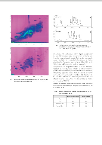
Fig. 3 Scheme of the LCxLC-Assist software Fig. 5 Analysis of a red wine sample. A comparison of the
µL empty loops).
second-dimension separation of the 65 fraction for both
th
B LC×LC plots shown in Fig. 4A–B.
2-3. Software
4. Results and Discussion
4. Results and Discussion
• Shimadzu LabSolutions (Version 5.60 SP2) An evaluation of the performance, in terms of peak capacity (n C ), of
In an LC×LC system, with two not orthogonal dimensions, an the two different set-ups tested was carried out, considering both
LC×LC separation most likely results in peaks concentrated around theoretical and practical peak capacity. The theoretical peak capacity
2-4. 2D Software the main diagonal line of the separation area. A typical example is values, multiplicative of the individual values obtained for the two
1
2
• LCxLC-Assist the LC×LC analysis of a red wine sample, illustrated in Fig. 4A, by dimensions ( n C × n C ), yielded values as high as 690 and 570 for the
employing a Cyano column in the D1 and a C18 column in the D2 full in fraction and for the shifted gradients, respectively.
• ChromSquare (Version 2.0) from Chromaleont, Messina, Italy
using the conventional full-in-fraction approach.
As expected, due to the partial correlation of the two dimensions,
As a matter of fact, a clear correlation of the D1 and D2 and a small “practical” peak capacity values, corrected for both undersampling
3. LC×LC-MS Conditions peak-distribution area were observed because the separation mech- (number of fractions effectively transferred from the D1 to the D2) and
anisms in the two dimensions were similar. The analytes eluted early orthogonality (separation space effectively covered by sample
First dimension (D1) separations in the D1 were only weakly retained in the D2; the analytes eluted compounds), were signi¦cantly lower at 75 and 216. The set-up with
Column : Ascentis Cyano in the middle of the D1 were eluted in the middle of the D2 and the the use of the shifted second dimension gradients was the most
Flow rate : 20 µL/min
Mobile phases : ( A) 0.1% acetic acid in water (pH around 3); analytes eluted late in the D1 were strongly retained in the D2. Fig. 4 Separation of a red wine sample by using the FIF (A) and the ef¦cient one since it less suffered from the correlation of the two
(B) acetonitrile 0.1% acetic acid. shifted gradient (B) approaches dimensions tested (Table 1).
Gradient elution : 0.01 min, 2% B; 10 min, 2% B; 60 min, 50% B; 75 min, To overcome such a limitation, we used a narrower organic solvent
100% B; 100 min, 100% B. span changing the gradient program according to the elution prop- Selected ion extracted chromatograms for some target compounds
Backpressure (at analysis start) = 40 bar erties. The shifted gradient program, led to a greater coverage of occurring in the red wine sample along the relative mass spectra are
Injection volume : 5 mL
the separation space (Fig. 4B). The blue line is the program of the illustrated in Fig. 6.
Second dimension (D2) separations D1 run and the red line is that of the D2 run. The D2 gradient cov-
Column : Ascentis Express C18 ered a narrow organic solvent range, which varied continuously Table 1 Relative performances, in terms of peak capacity, n C , of the
Flow rate : 2.5 mL/min during the LC×LC run. The gradient program started with 0% ace- two set-up investigated
Mobile phases : ( A) 0.1% acetic acid in water (pH around 3);
(B) acetonitrile 0.1% acetic acid. tonitrile and rose to 20% ACN over 0.75 min; at the end of the Full in fraction gradient Shifted gradient
Gradient elution : analysis, the gradient program in the D2 starts at 10% acetonitrile
FIF, full in fraction: 0.01 min, 0% B; 0.10 min, 0% B; 0.75 min, and rose to 50% acetonitrile. At the end of the analysis, the higher 1 n C 15 15
50% B; 1.00 min, 0% B.
SG, Shifted gradient: illustrated in Fig. 3 percentage of organic solvent made possible the ef¦cient elution of 2 n C 46 38
Backpressure (at analysis start) = 170 bar the strongly retained compounds. Theoretical D2 n C 690 570
Modulation time of the switching valves : 1 min.
As can be seen from Fig. 4B regarding the red wine sample analyzed Practical D2 n C 75 216
with LC×LC with a shifted gradient in the D2, a signi¦cant improve-
MS conditions
ment in the retention space was attained (Fig. 5). In fact, the use of
MS acquisition performed using the ESI interface operating in negative a shifted gradient with a gradual increase of the proportion of or-
ionization mode:
ganic solvent gave better separation in the D2 with a less typical di-
mass spectral range: 100–800 m/z; event time: 0.1 sec; scan speed:
agonal-line distribution. In addition, because of the narrower sol-
7500 u/s; nebulizing gas (N 2 ) ow: 2 L/min; drying gas (N 2 ) ow: 15 vent range, the backpressure was much smoother and steadier.
L/min; Heat block temperature: 250 °C; desolvation line (DL) tempera-
ture: 250 °C; Interface voltage: 3.5 kV; detector voltage: 1.80 kV; The
ow eluting from the second column was splitted before the MS in-
strument (approximately 0.4 mL/min to the MS).

2