Page 22 - Shimadzu Journal vol.9 Issue1

Clinical Research

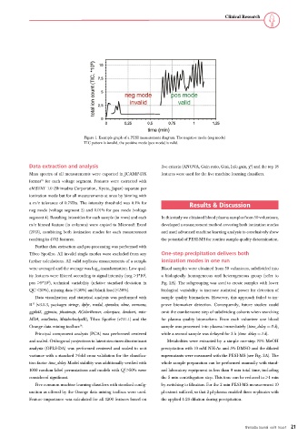
Figure 1. Example graph of a PESI measurement diagram. The negative mode (neg mode)
TIC pattern is invalid, the positive mode (pos mode) is valid.

Data extraction and analysis five criteria (ANOVA, Gain ratio, Gini, Info.gain, χ ) and the top 18
2
Mass spectra of all measurements were exported in JCAMP-DX features were used for the five machine learning classifiers.
format for each voltage segment. Features were extracted with
16
eMSTAT 1.0 (Shimadzu Corporation, Kyoto, Japan) separate per
ionization mode but for all measurements at once by binning with
a m/z tolerance of 0.75Da. The intensity threshold was 0.1% for Results & Discussion
neg mode (voltage segment 2) and 0.01% for pos mode (voltage
segment 4). Resulting intensities for each sample (in rows) and each In this study we obtained blood plasma samples from 50 volunteers,
m/z binned feature (in columns) were copied to Microsoft Excel developed a measurement method covering both ionization modes
(2013), combining both ionization modes for each measurement and used advanced machine learning analysis to conclusively show
resulting in 4702 features. the potential of PESI-MS for routine sample-quality determination.
Further data extraction and pre-processing was performed with
Tibco Spotfire. All invalid single modes were excluded from any One-step precipitation delivers both
further calculations. All valid replicate measurements of a sample ionization modes in one run
were averaged and the average was log -transformation. Low qual- Blood samples were obtained from 50 volunteers, subdivided into
10
3
ity features were filtered according to signal intensity (neg >1*10 , a biologically homogeneous and heterogeneous group (refer to
pos >9*10 ), technical variability (relative standard deviation in Fig. 2A). The subgrouping was used to create samples with lower
3
QC <50%), missing data (<30%) and blank load (<50%). biological variability to increase statistical power for detection of
Data visualization and statistical analysis was performed with sample quality biomarkers. However, this approach failed to im-
17
R (v3.5.3, packages stringr, dplyr, readxl, openxlsx, nlme, emmeans, prove biomarker detection. Consequently, future studies could
ggplot2, ggpmisc, pheatmap, RColorBrewer, colorspace, dendsort, miss- omit the cumbersome step of subdividing cohorts when searching
MDA, mixOmics, MetaboAnalystR), Tibco Spotfire (v7.11.1) and the for plasma quality biomarkers. From each volunteer one blood
18
Orange data mining toolbox . sample was processed into plasma immediately (time_delay = 0 h),
Principal component analysis (PCA) was performed centered while a second sample was delayed for 3 h (time_delay = 3 h).
and scaled. Orthogonal projections to latent structures discriminant Metabolites were extracted by a simple one-step 70% MeOH
analysis (OPLS-DA) was performed centered and scaled to unit precipitation with 10 mM NH4Ac and 5% DMSO and the diluted
variance with a standard 7-fold cross validation for the classifica- supernatants were measured with the PESI-MS (see Fig. 2A). The
tion factor time_delay. Model stability was additionally verified with whole sample preparation can be performed manually with stand-
2
1000 random label permutations and models with Q >50% were ard laboratory equipment in less than 8 min total time, including
considered significant. the 5 min centrifugation step. This time can be reduced to >1 min
Five common machine learning classifiers with standard config- by switching to filtration. For the 2 min PESI-MS measurement 10
uration as offered by the Orange data mining toolbox were used. µl extract sufficed, so that 2 µl plasma enabled three replicates with
Feature importance was calculated for all 1200 features based on the applied 1:20 dilution during precipitation.

21
Shimadzu Journal vol.9 Issue1 21